WUFI® 2D computes the time-dependent temperature and moisture fields in a two-dimensional cross-section of a building component. Such a two-dimensional computation automatically includes so-called geometrical and structural thermal bridge effects. These are the effects which the component shape (e.g. a corner) and variations of the thermal properties within the component (e.g. reinforcement bars) have on the resulting temperature field. The modifications of the temperature field and the associated heat flows by thermal bridges may have important consequences for energy loss, mold growth in damp corners etc.
WUFI® 2D is not intended to compete with dedicated thermal bridge programs which usually offer more flexible modelling interfaces and provide specific thermal bridge properties. But it can investigate the effect of thermal bridges on energy losses and, in particular, on the hygric conditions in and on building components (mold growth, damage due to condensation etc.), which purely thermal programs can not.
The international standard ISO 10211 provides a series of two- and three-dimensional test cases for validating thermal bridge software. Of course, WUFI® 2D should be able to reproduce the two-dimensional test cases.
Test case 1
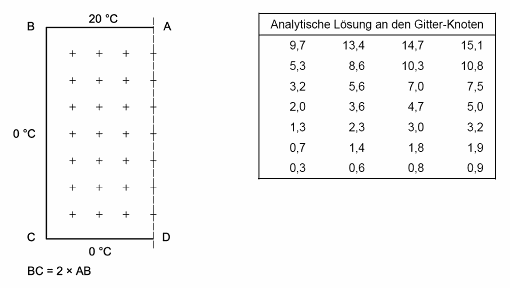
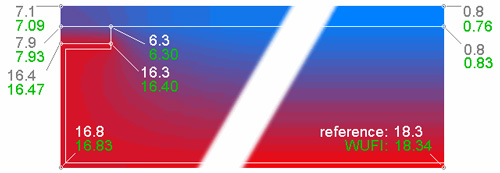
Case 1 considers one half of a symmetrical square column with known constant surface temperatures. The steady-state temperature distribution over the cross-section can be computed analytically. 28 temperatures on an equidistant grid are given by the standard as the reference solution; the software to be validated must reproduce these temperatures within 0.1° C.
 The given boundary conditions (20° C along the top edge, 0° C along the left and bottom edges, and adiabatic along the right edge) result in a temperature field with strong variation close to the upper left corner and little variation towards the bottom of the cross-section.
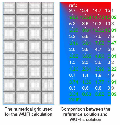
Usually, one would therefore create a more efficient variable-size computational grid with fine grid elements close to the upper left corner and progressively larger grid elements towards the bottom. However, since for the present purpose the temperatures must be evaluated at precisely given coordinates and WUFI® computes the temperatures for the centers of the grid elements, a grid has to be created which ensures that a small element is centered at each of the requested positions.
To this end, the monolithic component has been built up from 28 separate blocks which fill up the space between the reference points and are subdivided by relatively coarse grids. The blocks are separated by 4 mm wide gaps which are subdivided by very fine grids in such a way that one small grid element is precisely centered on each reference point (one at each intersection of the gaps).
Since in the present case of a monolithic component with given surface temperatures the steady-state solution for the temperature field does not depend on the thermal properties, any arbitrary material data may be used. The data of concrete were chosen for this exercise.
The prescribed surface temperatures are applied to the component by setting the ambient air to the desired temperatures and the heat transfer coefficients for the surfaces to very large values. For the adiabatic right-hand surface (the symmetry plane which allows to limit the calculation to one half of the original square column), the heat transfer coefficient has been set to zero in order to suppress any heat exchange.
WUFI® 2D has no mode for steady-state solutions, but such a solution is approached to arbitrary precision if a transient computation with constant boundary conditions is performed for a sufficient number of time steps. Here, 10 steps of 48 hours each were found to be sufficient. Moisture transport was switched off for this purely thermal computation.
A graphical postprocessor for the calculation results allows to extract the final temperatures from any grid element. The comparison with the reference temperatures shows that WUFI’s temperatures deviate by 0.05° C or less and are thus well within the allowed deviation of 0.1° C.
You can download a WUFI® 2D project file (65 KB) for the benchmark calculation. Use the “Import…” function of WUFI® 2D to read this compressed archive file.
Test case 2
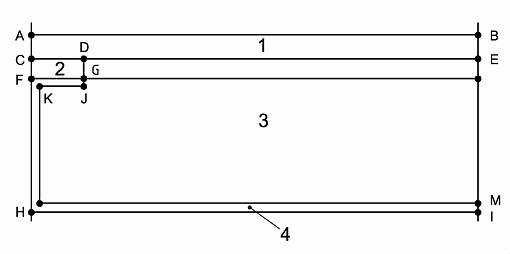
Case 2 considers the heat flow through a building component which contains materials with widely differing thermal conductivities.
| Dimensions (mm): | ||||||
| AB= 500 | CD = 15 | EM = 40 | IM = 1.5 | |||
| AC = 6 | CF = 5 | GJ = 1.5 | FG-KJ = 1.5 | |||
| Thermal conductivities (W/mK): | ||||||
| 1 (concrete): 1.15 | 2 (wood): 0.12 | 3 (insulation): 0.029 | 4 (aluminum): 230 | |||
| Boundary conditions: | |||
| AB: 0° C with Rse = 0.06 m²K/W | HI: 20° C with Rsi = 0.11 m²K/W | ||
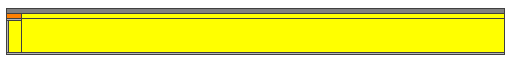
The prescribed building component can easily be assembled from rectangles, using WUFI’s graphical component editor. The automatically generated grid with the fineness setting “coarse” is sufficient for this computation.
The thermal conductivities for the four involved materials are specified by the standard and have been entered in WUFI® accordingly. Since WUFI® needs a full set of thermal porperties for each material (including heat capacity etc.) the missing data have been taken from similar materials in WUFI’s material database. The steady-state result only depends on the prescribed thermal conductivities, not on the added properties.
The ambient air temperatures and the heat transfer coefficients for the top and bottom surfaces are entered in WUFI® 2D as specified by the standard. The left and right surfaces are treated as adiabatic by setting the respective heat transfer coefficients to zero.
In this case, too, the steady-state solution must be approximated by a transient calculation with constant boundary conditions. 30 steps of one hour each were found sufficient.
The resulting temperatures at the specified locations can again be extracted with the graphical postprocessor. However, the standard asks for temperatures on material boundaries whereas WUFI® computes the temperatures for the centers of the grid elements and any material boundaries must always coincide with boundaries between grid elements. So in this case it is not possible to center grid elements on the requested locations (such grid elements would contain two or more different materials which is not allowed).
Close to the four corners (points A, B, H and I), the temperature variation is so small that the center of the outermost grid element instead of the true geometric corner can be taken as sufficiently representative.
Where the requested location lies between two materials (points C, E and F), the temperature at this location must be computed from the temperatures at the centers of the two grid elements straddling the location. The temperature ϑm for a location m between locations 1 and 2 can be computed by ϑm = ((λ1/s1) ϑ1 + (λ2/s2) ϑ2) / ((λ1/s1)+(λ2/s2)), where ϑi is the temperature at location i, λi is the thermal conductivity between locations i and m, and si is the distance between locations i and m. Since the grid elements straddling a material boundary all have the same size, the si cancel and the expression reduces to ϑm = (λ1 ϑ1 + λ2 ϑ2) / (λ1+λ2).
For locations where three materials meet (points D and G), the temperature has been computed from the temperatures in the four adjacent grid elements by the following generalisation of the above formula: ϑm = (λ1 ϑ1 + λ2 ϑ2 + λ3 ϑ3 + λ4 ϑ4) / (λ1 + λ2 + λ3 + λ4).
The comparison with the reference temperatures shows that WUFI’s temperatures deviate by 0.1° C or less and are thus within the allowed deviation of 0.1° C. The heat flow through the component is 9.5 W/m and thus within the required (9.5 ± 0.1) W/m.
You can download a WUFI 2D project file (30 KB) for the benchmark calculation. Use the “Import…” function of WUFI® 2D to read this compressed archive file.
Last Update: September 18, 2025 at 9:06